Repeating your Coordinate System

A very useful operation in fragment shader development is repeating a coordinate system. It’s also quite neat since we’re able to draw several shapes without the use of a loop. When working in 3D and raymarching it’s extra awesome because we can fake the repetition of infinite shapes into a space. Here I discuss one method of performing this repetition task.

First let’s create a simple framework:

float sdCircle(vec2 p, float r){
  return length(p)-r;
}

void main(){
  vec2 p = (gl_FragCoord.xy/u_res)-0.5;
  float i = step(sdCircle(p, .5), 0.);
  gl_FragColor = vec4(vec3(i),1);
}

We define a vector for each fragment that ranges from -.5 from the bottom left corner to +.5 to the top right with a zero vector in the middle of the canvas.

We define a function to calculate the distance from p to the center of the circle, using step will make the intensity variable (i) either 0 or 1.

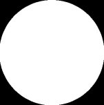
It yields a happy circle:

Let’s say we want to repeat this circle 4 times. We’ll need to create a vector that repeats across the canvas several times. To help with this, we’ll use mod().

Now the span of the current coordinate system is 1 (-.5 to +.5) so if we want 4 cells, we should use mod(p, .25) ….or better yet mod(p, 1/4) which is slightly more intuitive. We’ll also need to adjust the radius of the circles so they fit in the new cell sizes. Let’s make them half the cell size.

  float cellSz = 1./4.;
  float r = cellSz/2.;
  p = mod(p, vec2(cellSz));
  float i = step(sdCircle(p, r), 0.);

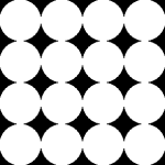
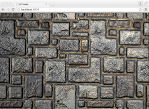
It gives us:

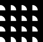
Wait, what’s this? Why are the circles cut off and no longer happy?

Well, remember how we used mod? mod returns positive values–in our case: 0 to .25. This means that for the variable p, the bottom left corner is (0,0) and the very top is (.25, .25)

What we actually want is ‘centered’ ranges from vec2(-.125) to vec2(.125), right? But wait! We already did this! At the start of main we divided the fragCoord by resolution then subtracted .5. We just need to do something similar. In this case, subtract half of whatever the cell size is.

  p = mod(p, vec2(cellSz))-vec2(0.5*cellSz);

Now our circles are happy again!

length, distance, sqrt

I was really amazed the first time I saw a similar visualization on the Processing homepage…err, like 10 years ago. It’s such a simple concept, but very pretty. Anyway, I finally sat down and gave it a go in glsl. While working with it I played around with the distance calculations and figured I should write a tiny bit about that.

When you need to calculate the distance between two points, you have a few options. You can write a function yourself, or use one of the built-in functions in glsl: distance(), length(), or sqrt(). distance() takes in two vectors. length() accepts 1 vector and sqrt() takes in a float (typically). But sometimes you don’t need the exact distance. Sometimes you’re just trying to find out if the length of a vector is longer than some defined value. In these situations you can use the squared distance instead.

For the squared distance you just need to get the difference between vector A and B then assign to say, C. The squared distance would then be: c.x*c.x+c.y*c.y. Or even: dot(c,c); So basically it’s everything length does without the call to sqrt–which is the computationally expensive part.

The values returned from these two methods (sqrt distance and squared distance) are of course fundamentally different, so you’ll need to adjust the value you are comparing against if you switch between the two.

Making Infinity

Creating an infinite-like shape is really easy. Set the x component of the position of the object to be cos(time). This will make the object oscillate back and fourth along the x axis. Then set the y component to use sin(time*2). By multiplying by 2, it doubles the frequency. At this point, you’ll probably want to scale down the amplitude of the y since the infinity shape is longer than it is tall. Try values between 2 or 3:
y = sin(time*2)/2.5

What happens if you set x=cos(time) and y=sin(time)? Try it out! Play around with the values to see what other fun patterns you can make!

Visualizing SDFs: Flies & Force Fields

I’ve been spending quite a bit of time learning shaders and with that, learning SDFs (Signed Distance Functions). SDFs are very useful for rendering geometric shapes. There’s certainly a beauty to them–composed basically of just a bunch of math. Often void conditionals, they are efficient, but not so readable.

When first learning to read SDFs, it can be daunting. Just take a look at the definition for a cylinder:

float sdCylinder(vec3 p, vec2 sz ){
  vec2 d = abs(vec2(length(p.xz),p.y)) - sz;
  float _out = length(max(vec2(d.x,d.y), 0.));
  float _in = min(max(d.x,d.y), 0.);
  return _in + _out;
}

Errr, what? A month ago, I would have given up after the second line. Certain visualization tools are necessary to help break apart the logic, which is what this blog is all about.

Anyway, this week I was in process of understanding a cylinder SDF and I had a neat insight. Understanding the logic is much easier if visualized with flies and force fields.

Game Rules

In this world, our object is enveloped in force fields. Each field has a fly trapped inside. Poor dudes. Flies cannot pass between the fields. There’s the “tube” force field that defines the radius of the cylinder and force fields along the XZ-planes controlling the height.

There’s also a fly trapped inside the object itself and another stuck directly on the cylinder. Other than not being able to pass between fields, the flies (our sample points) are free to travel anywhere inside the field. And each case, there is a straight-line distance from the fly/point to the object. The force fields represent the different cases of our logic. Hmmm, a diagram might help:

If you spend a bit of time visualizing each case separately, seeing the flies buzzing in their respective fields, it becomes more clear how the different parts of the logic work.

Fly A: (y – height) => (Cylinder Top)
Fly B: length of vec2(p.xz – radius, p.y – height) => (Cylinder Rim)
Fly C: length of (p.xz – radius) => (Cylinder Body)
Fly D: greater of length of (p.xz – radius) OR (y-height) => (Inside Cylinder)
Fly E: distance = zero, strictly lives on cylinder

Okay, let’s dive in.

float sdCylinder(vec3 p, vec2 sz ){

Easy stuff here. Return a float since which is our distance from the sample point to the surface of the object. The two parameters are a vec3 p and a vec2 sz. The sz variable contains the radius and height of the cylinder as its x and y components respectively.

vec2 d = abs(vec2(length(p.xz),p.y)) - sz;

The vec2 defined contains p.xz distance from the origin and p.y. We use abs since a cylinder is symmetrical and only the “top right front” part needs to be evaluated. Everything else is just a “mirror” case. Subtracting sz yields the differences for both the “top” and “body” distances. Store that in d.

float _out = length(max(vec2(d.x, d.y), 0.));

Using max with zero isolates which case we’re working with. If the point/fly is at the top of the cylinder, then d.x < 0. If it is in the ‘body’ force field, it’s d.y 0 and d.y > 0, the we’re dealing with fly B. The neat part is that either we’ll have one component set to zero in which case length is just using 1-dimensions, or we’ll have 2 components, which case length still works.

float _in = min(max(d.x,d.y), 0.);

Lastly, if the fly is trapped inside, then which surface is it closer to? Top or body? d.y or d.x? Use max to find that out. If one of the values are positive here, min is used to set it to zero. Think of min here as a replacement to a conditional.

Again, here is the final definition:

float sdCylinder(vec3 p, vec2 sz ){
  vec2 d = abs(vec2(length(p.xz),p.y)) - sz;
  float _out = length(max(vec2(d.x,d.y), 0.));
  float _in = min(max(d.x,d.y), 0.);
  return _in + _out;
}

This visualization tool has helped me to deconstruct the SDF logic. I hope it has been of use to you too! I suggest memorizing the five cases where the fly/point can exist. Then you can derive the code from scratch if necessary–it’s a good way of testing your understanding. It’s also really fun once you grasp it!

Normal Mapping using PShaders in Processing.js

Try my normal mapping PShader Demo:

Last year I made a very simple normal map demo in Processing.js and I posted it on OpenProcessing. It was fun to write, but something that bothered me about it was that the performance was very slow. The reason for this was because it uses a 2D canvas–there’s no hardware acceleration.

Now, I have been working on adding PShader support into Processing.js on my spare time. So here and there i’ll make a few updates. After fixing a bug in my implementation recently, I had enough to port over my normal map demo to use shaders. So, instead of having the lighting calculations in the sketch code, I could have them in GLSL/Shader code. I figured this should increase the performance quite a bit.

Converting the demo from Processing/Java code to GLSL was pretty straightforward–except working out a couple of annoying bugs–I got the demo to resemble what I originally had a year ago, but now the performance is much, much, much better 🙂 I’m no longer limited to a tiny 256×256 canvas and I can use the full client area of the browser. Even with specular lighting, it runs at a solid 60 fps. yay!

If you’re interested in the code, here it is. It’s also posted on github.

#ifdef GL_ES
precision mediump float;
#endif

uniform vec2 iResolution;
uniform vec3 iCursor;

uniform sampler2D diffuseMap;
uniform sampler2D normalMap;

void main(){
	vec2 uv = vec2(gl_FragCoord.xy / 512.0);
	uv.y = 1.0 - uv.y;

	vec2 p = vec2(gl_FragCoord);
	float mx = p.x - iCursor.x;
	float my = p.y - (iResolution.y - iCursor.y);
	float mz = 500.0;

	vec3 rayOfLight = normalize(vec3(mx, my, mz));
	vec3 normal = vec3(texture2D(normalMap, uv)) - 0.5;
	normal = normalize(normal);

	float nDotL = max(0.0, dot(rayOfLight, normal));
	vec3 reflection = normal * (2.0 * (nDotL)) - rayOfLight;

	vec3 col = vec3(texture2D(diffuseMap, uv)) * nDotL;

	if(iCursor.z == 1.0){
		float specIntensity = max(0.0, dot(reflection, vec3(.0, .0, 1.)));
		float specRaised = pow(specIntensity, 20.0);
		vec3 specColor = specRaised * vec3(1.0, 0.5, 0.2);
		col += specColor;
	}

	gl_FragColor = vec4(col, 1.0);
}

Experimenting with Normal Mapping using PShaders

Just over half a year ago, I wrote a blog about Experimenting with Normal Mapping. I wrote a simple Processing sketch that demonstrated the technique and I also wrote a hacked up Processing.js sketch to squeeze out some extra few frames/sec on the browser side of things.

This long weekend, I found myself with some extra time to hack on something. I remember that several weeks ago, Processing 2 introduced PShaders, which at the time I found exciting, but I didn’t have a chance to look at them. So this weekend I decided to take a look into this new PShader object. I haven’t touched shaders in a while, so I brushed up on them by reading the PShader tutorial on the Processing page.

After my refresher, I got to hacking and re-wrote my normal mapping sketch. Here is my complete sketch along with vertex and fragment shaders:

The sketch:

PImage diffuseMap;
PImage normalMap;

PShape plane;

PShader normalMapShader;

void setup() {
  size(256, 256, P3D);
  
  diffuseMap = loadImage("crossColor.jpg");
  normalMap = loadImage("crossNormal.jpg");
  
  plane = createPlane(diffuseMap);
  
  normalMapShader = loadShader("texfrag.glsl", "texvert.glsl");
  shader(normalMapShader);
  normalMapShader.set("normalMap", normalMap);
}

void draw(){
  background(0);
  translate(width/2, height/2, 0);
  scale(128);
  shape(plane);
}

void mouseMoved(){
  updateCursorCoords();
}

void mouseDragged(){
  updateCursorCoords();
}

void updateCursorCoords(){
  normalMapShader.set("mouseX", (float)mouseX);
  normalMapShader.set("mouseY", height - (float)mouseY);
}

void mousePressed(){
  normalMapShader.set("useSpecular", 1);
}

void mouseReleased(){
  normalMapShader.set("useSpecular", 0);
}

PShape createPlane(PImage tex) {
  textureMode(NORMAL);
  PShape sh = createShape();
  sh.beginShape(QUAD);
  sh.noStroke();
  sh.texture(tex);
  sh.vertex( 1, -1, 0, 1, 0);
  sh.vertex( 1,  1, 0, 1, 1);    
  sh.vertex(-1,  1, 0, 0, 1);
  sh.vertex(-1, -1, 0, 0, 0);
  sh.endShape(); 
  return sh;
}

The vertex shader:

#define PROCESSING_TEXTURE_SHADER

uniform mat4 transform;
uniform mat4 texMatrix;

attribute vec4 vertex;
attribute vec2 texCoord;

varying vec4 vertTexCoord;

void main() {
  gl_Position = transform * vertex;
  vertTexCoord = texMatrix * vec4(texCoord, 1.0, 1.0);
}

The fragment shader:

#ifdef GL_ES
precision mediump float;
precision mediump int;
#endif

#define PI 3.141592658

uniform sampler2D normalMap;
uniform sampler2D colorMap;

uniform int useSpecular;

uniform float mouseX;
uniform float mouseY;

varying vec4 vertTexCoord;

const vec3 view = vec3(0,0,1);
const float shine = 40.0;

void main() {
  // Convert the RGB values to XYZ
  vec4 normalColor  = texture2D(normalMap, vertTexCoord.st);
  vec3 normalVector = vec3(normalColor - vec4(0.5));
  normalVector = normalize(normalVector);

  vec3 rayOfLight = vec3(gl_FragCoord.x - mouseX, gl_FragCoord.y - mouseY, -150.0);
  rayOfLight = normalize(rayOfLight);

  float nDotL = dot(rayOfLight, normalVector);

  vec3 finalSpec = vec3(0);

  if(useSpecular == 1){
    vec3 reflection = normalVector;
    reflection = reflection * nDotL * 2.0;
    reflection -= rayOfLight;
    float specIntensity = pow( dot(reflection, view), shine);
    finalSpec = vec3(1.0, 0.5, 0.2) * specIntensity;
  }

  float finalDiffuse = acos(nDotL)/PI;

  gl_FragColor = vec4(finalSpec + vec3(texture2D(colorMap, vertTexCoord.st) * finalDiffuse), 1.0);
}

Performance

I found using PShaders very exciting, since I could place all this computational work on the GPU rather than CPU. So I wondered about the performance vs my old sketch. I’m on a mac mini, and after running tests I found my original normal mapping sketch ran at 30FPS with diffuse lighting and it ran at 21FPS using diffuse and specular lighting. Using PShaders, I was able to render specular and diffuse lighting at a solid 60FPS. Keep in mind the first sketch is 2D and my new one is 3D, so I’m not sure if that comparison is fair.

No Demo? 😦

Sadly, Processing no longer allows exporting to applets, so I can’t even post a demo running in Java. The perfect solution would be to implement the PShader in Processing.js, which is something I’m considering….