On Writing Software

It’s surprising how much of programming is actually just coming up with metaphors, paradigms, and verbs to shape the code’s meaning and intent.

The same old data structures repeated over and over….but it’s the treatment of the structures is what seems to give those structures life, context, and meaning. Also known as patterns.

Patterns take the collection of abstract variables–which could represent potentially anything–and put them into a world in which the developer has understanding. A world with constraints and logic. It’s the marriage between pure logic and the emotional human mind.

One of the joys of writing code is playing multi-layer see-saw with pure math: min, max, sin, cos.
Then bundling those operations into nodes within structures: graphs, trees, lists.
Then later applying some constraints on the structures to form patterns: factories, events, composites.
Finally adding business logic constraints. (btw, I don’t mean the ‘yucky’ definition of business–that’s boring.)

Now the code has gained life inside a virtual world. The entire process is incredibly fascinating, but I feel the final process–where the code begins to take on life–is the most interesting.

The execution occurs on the CPU, but the concepts live inside the mind of the developer who has written them. It’s as if the code is present in two places at once: inside the brain of the computer and the mind of a human.

This is one of the reasons why I enjoy writing code so much. There’s a concept, entirely abstract that gets translated into discrete binary operations, entirely concrete.

I find this whole procedure very fascinating.

Repeating your Coordinate System

A very useful operation in fragment shader development is repeating a coordinate system. It’s also quite neat since we’re able to draw several shapes without the use of a loop. When working in 3D and raymarching it’s extra awesome because we can fake the repetition of infinite shapes into a space. Here I discuss one method of performing this repetition task.

First let’s create a simple framework:

float sdCircle(vec2 p, float r){
  return length(p)-r;
}

void main(){
  vec2 p = (gl_FragCoord.xy/u_res)-0.5;
  float i = step(sdCircle(p, .5), 0.);
  gl_FragColor = vec4(vec3(i),1);
}

We define a vector for each fragment that ranges from -.5 from the bottom left corner to +.5 to the top right with a zero vector in the middle of the canvas.

We define a function to calculate the distance from p to the center of the circle, using step will make the intensity variable (i) either 0 or 1.

It yields a happy circle:
repeat_circle

Let’s say we want to repeat this circle 4 times. We’ll need to create a vector that repeats across the canvas several times. To help with this, we’ll use mod().

Now the span of the current coordinate system is 1 (-.5 to +.5) so if we want 4 cells, we should use mod(p, .25) ….or better yet mod(p, 1/4) which is slightly more intuitive. We’ll also need to adjust the radius of the circles so they fit in the new cell sizes. Let’s make them half the cell size.

  float cellSz = 1./4.;
  float r = cellSz/2.;
  p = mod(p, vec2(cellSz));
  float i = step(sdCircle(p, r), 0.);

It gives us:
repeat_2.png

Wait, what’s this? Why are the circles cut off and no longer happy?

Well, remember how we used mod? mod returns positive values–in our case: 0 to .25. This means that for the variable p, the bottom left corner is (0,0) and the very top is (.25, .25)

What we actually want is ‘centered’ ranges from vec2(-.125) to vec2(.125), right? But wait! We already did this! At the start of main we divided the fragCoord by resolution then subtracted .5. We just need to do something similar. In this case, subtract half of whatever the cell size is.

  p = mod(p, vec2(cellSz))-vec2(0.5*cellSz);

Now our circles are happy again!
repeat_3

length, distance, sqrt

coonextions.gif

I was really amazed the first time I saw a similar visualization on the Processing homepage…err, like 10 years ago. It’s such a simple concept, but very pretty. Anyway, I finally sat down and gave it a go in glsl. While working with it I played around with the distance calculations and figured I should write a tiny bit about that.

When you need to calculate the distance between two points, you have a few options. You can write a function yourself, or use one of the built-in functions in glsl: distance(), length(), or sqrt(). distance() takes in two vectors. length() accepts 1 vector and sqrt() takes in a float (typically). But sometimes you don’t need the exact distance. Sometimes you’re just trying to find out if the length of a vector is longer than some defined value. In these situations you can use the squared distance instead.

For the squared distance you just need to get the difference between vector A and B then assign to say, C. The squared distance would then be: c.x*c.x+c.y*c.y. Or even: dot(c,c); So basically it’s everything length does without the call to sqrt–which is the computationally expensive part.

The values returned from these two methods (sqrt distance and squared distance) are of course fundamentally different, so you’ll need to adjust the value you are comparing against if you switch between the two.

Deconstructing Voxel Rendering

mc

For someone who is fairly obsessed with pixel art, it isn’t a surprise I really like voxel rendering, too.

I feel I finally reached the point where I have enough knowledge about shader code that I can start to deconstruct voxel shaders to understand them. So I began to do just that. I started with a simple shader on ShaderToy, took it apart and put it back together. I renamed variables, made some changes, simplified some things, etc.

Here is the shader on shadertoy. The original source from where I got the code is posted at the top of the shader.
https://www.shadertoy.com/view/4lKyDW

Okay, so let’s dig in.

Define some constants. Nothing too special here. MAX_STEPS is used for raymarching. Grass and Dirt are colors obviously.

const float MAX_STEPS = 1000.;
const float GrassHeight = 0.8;
const vec3 Grass = vec3(.2, 1, 0);
const vec3 Dirt = vec3(.5,.25, 0);

Just a main(), no magic yet…

void mainImage(out vec4 fragColor, in vec2 fragCoord) {

Okay, we’re raymarching right? That means, we’ll need to define the ray start position. We can set x to whatever. It doesn’t really matter. The y component needs to be a large enough value so we can see the terrain. Z is set to simulation time so that the flyover seems animated.

vec3 rayOrigin = vec3(0., 12, iDate.w*5.);

Normalize the screenspace coords. We’ll need this in a couple places later on.

vec2 pnt = fragCoord.xy/iResolution.xy*2.-1.;

The ray direction. Unlike the ray origin, the ray direction varies slightly for each fragment–spreading out from -1 to 1 on the xy plane. Note z points positive 1.

vec3 rayDir = vec3(pnt, 1.);

Define the final color that we’ll assign to this particular fragment.

vec3 color;

The purpose of depth is to scale the ray direction vector.

float depth = 0.;

Okay, we reached the raymarching loop.

for(float i = .0; i < MAX_STEPS; ++i) { 

Since the top part of the screen space is empty, it makes sense to add a check early on to exit if we know the ray won’t actually hit anything. Of course this might need to be adjusted if the rayOrigin changes.

  if(pnt.y > 0.){
    break;
  }

Pretty standard raymarching stuff. We start with the origin and scale the ray direction a bit longer every iteration. The first iteration depth is zero, so we’d just be using the rayOrigin.

  vec3 p = rayOrigin + (rayDir * depth);

Okay, now we finally come to something that’s necessarily the ‘voxel’ part of the rendering. By flooring p we are ‘snapping’ the calculated raymarched point to the nearest 3D box/grid/cell.
Scaling the floored value by a smaller number will yield a higher ‘resolution’.

  vec3 flr = floor(p) * 0.25;

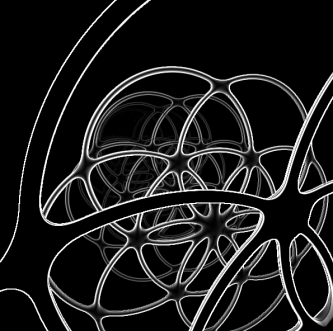
Okay, let’s take our attention to the wave-like pattern of the terrain. There are peaks and there are valleys. These are of course generated by using cos() and sin(). The waves created are the interactions/addition of the functions along the space.

This is where we decide if we are going to set the color of the fragment. If the floored y value is less then the cos()+sin(), then we want to color the fragment. Otherwise it means the y is higher so keep iterating.

  if(flr.y < cos(flr.z) + sin(flr.x)){
  
  frct = fract(p);
  if(frct.y > GrassHeight){
    color = Grass;
  }
  else{
    color = Dirt;
  }

If we hit a voxel and set the color, there’s no need to keep iterating. Break out of the loop.

    break;
  }// close the if

Depth is used to scale the ray direction, so we increment it a tiny bit every iteration. Since i ranges from 0 to 1000 and since we are scaling i here, the ray direction will scale from .0 to .1

  depth += i * (.1/MAX_STEPS);
}

We need to add some lighting, even if really fake to give the illusion of distance. It also helps to hide some of the aliasing that happens at the very far points in the terrain.

If we exited the loop early on, depth will be a relatively small value which means the fragments will end up being bright.
The farther it took to hit something, the darker that fragment will be. Play around with this value for some interesting lighting effects.

  color *= 1./(depth/5.);
  fragColor = vec4(color, 1);
}

If you understood most of this try substituting the cos() and sin() functions with noise values. It will make some really fun variation in the terrain.

Making Infinity

i2.gif

Creating an infinite-like shape is really easy. Set the x component of the position of the object to be cos(time). This will make the object oscillate back and fourth along the x axis. Then set the y component to use sin(time*2). By multiplying by 2, it doubles the frequency. At this point, you’ll probably want to scale down the amplitude of the y since the infinity shape is longer than it is tall. Try values between 2 or 3:
y = sin(time*2)/2.5

What happens if you set x=cos(time) and y=sin(time)? Try it out! Play around with the values to see what other fun patterns you can make!

mix()

ezgif-5-b890251356.gif

mix() is a glsl function that allows you to linearly interpolate between two values. The math behind it is straightforward and I use it a lot for colors and vectors–but when applied to SDFs—well it’s almost magic the way it shape-shifts between two objects. With just 1 line of code!

Take a look:
mix(Box(p, size), Sphere(p, rad), sin(time));

The third variable in mix can be all sorts of interesting things: time, fractional part of time, sin, cursor position, z position in a scene,….It’s fun to play around with values that might not seem like they should be passed into the function. 😛

You can learn more about mix() on the Khronos reference pages:
https://www.khronos.org/registry/OpenGL-Refpages/gl4/html/mix.xhtml

Everything, Nothing, Infinity and Imperfection

Screen Shot 2018-07-21 at 12.22.12 PM.png

108 days ago I started a project where I would create a shader and post it online. Every day. Whatever I had that day, even if incomplete, would get posted. My primary goal was to learn how to write shaders. By the way, all my sketches live in a github repo: https://github.com/asalga/fragments
and my posts exist as videos on IG: https://www.instagram.com/andor_saga

My secondary goal was to (mostly) overcome perfection. I knew my sketches wouldn’t be exactly what I’d like them to be.  Well, they are actually far, far from what I’d like to be able to do.

The main goal was to learn shaders, the second goal, which I feel has been eating away at my life and happiness is the need for perfection. So sometimes I would create sketches, that were terrible, but I had to accept them as they were, their imperfections, and ultimately, my own imperfection. It’s been difficult. And sometimes I feel it’s impossible. I think I’ve gotten better? There’s certainly more things I do and leave as imperfect. Like, blogging for instance. I don’t really care about grammar or spelling as much as I used to. They are certainly important for some things, but beating myself up over trying to portray that I’m perfect at spelling and grammar–is a waste of energy.

I feel like I learned A LOT when it comes to shaders. I learned SDFs, SDF operations (intersections, unions, repetition), glsl syntax, …I would sometimes get these incredible insights, I started being able to vizualize 3D objects and rotate them in my mind. I was never able to do that before. It’s been a lot of fun. And I hope to continue making more sketches.

In terms of acceptace of imperfection, I think that’s going to be a life-long deal.

Visualizing SDFs: Flies & Force Fields

cylinder

I’ve been spending quite a bit of time learning shaders and with that, learning SDFs (Signed Distance Functions). SDFs are very useful for rendering geometric shapes. There’s certainly a beauty to them–composed basically of just a bunch of math. Often void conditionals, they are efficient, but not so readable.

When first learning to read SDFs, it can be daunting. Just take a look at the definition for a cylinder:

float sdCylinder(vec3 p, vec2 sz ){
  vec2 d = abs(vec2(length(p.xz),p.y)) - sz;
  float _out = length(max(vec2(d.x,d.y), 0.));
  float _in = min(max(d.x,d.y), 0.);
  return _in + _out;
}

Errr, what? A month ago, I would have given up after the second line. Certain visualization tools are necessary to help break apart the logic, which is what this blog is all about.

Anyway, this week I was in process of understanding a cylinder SDF and I had a neat insight. Understanding the logic is much easier if visualized with flies and force fields.

Game Rules

In this world, our object is enveloped in force fields. Each field has a fly trapped inside. Poor dudes. Flies cannot pass between the fields. There’s the “tube” force field that defines the radius of the cylinder and force fields along the XZ-planes controlling the height.

There’s also a fly trapped inside the object itself and another stuck directly on the cylinder. Other than not being able to pass between fields, the flies (our sample points) are free to travel anywhere inside the field. And each case, there is a straight-line distance from the fly/point to the object. The force fields represent the different cases of our logic. Hmmm, a diagram might help:

labels

If you spend a bit of time visualizing each case separately, seeing the flies buzzing in their respective fields, it becomes more clear how the different parts of the logic work.

dist

Fly A: (y – height) => (Cylinder Top)
Fly B: length of vec2(p.xz – radius, p.y – height) => (Cylinder Rim)
Fly C: length of (p.xz – radius) => (Cylinder Body)
Fly D: greater of length of (p.xz – radius) OR (y-height) => (Inside Cylinder)
Fly E: distance = zero, strictly lives on cylinder

Okay, let’s dive in.

float sdCylinder(vec3 p, vec2 sz ){

Easy stuff here. Return a float since which is our distance from the sample point to the surface of the object. The two parameters are a vec3 p and a vec2 sz. The sz variable contains the radius and height of the cylinder as its x and y components respectively.

vec2 d = abs(vec2(length(p.xz),p.y)) - sz;

The vec2 defined contains p.xz distance from the origin and p.y. We use abs since a cylinder is symmetrical and only the “top right front” part needs to be evaluated. Everything else is just a “mirror” case. Subtracting sz yields the differences for both the “top” and “body” distances. Store that in d.

float _out = length(max(vec2(d.x, d.y), 0.));

Using max with zero isolates which case we’re working with. If the point/fly is at the top of the cylinder, then d.x < 0. If it is in the ‘body’ force field, it’s d.y 0 and d.y > 0, the we’re dealing with fly B. The neat part is that either we’ll have one component set to zero in which case length is just using 1-dimensions, or we’ll have 2 components, which case length still works.

float _in = min(max(d.x,d.y), 0.);

Lastly, if the fly is trapped inside, then which surface is it closer to? Top or body? d.y or d.x? Use max to find that out. If one of the values are positive here, min is used to set it to zero. Think of min here as a replacement to a conditional.

Again, here is the final definition:

float sdCylinder(vec3 p, vec2 sz ){
  vec2 d = abs(vec2(length(p.xz),p.y)) - sz;
  float _out = length(max(vec2(d.x,d.y), 0.));
  float _in = min(max(d.x,d.y), 0.);
  return _in + _out;
}

This visualization tool has helped me to deconstruct the SDF logic. I hope it has been of use to you too! I suggest memorizing the five cases where the fly/point can exist. Then you can derive the code from scratch if necessary–it’s a good way of testing your understanding. It’s also really fun once you grasp it!

SDFs: Rendering a Rectangle

A couple of weeks ago I wrote a post on how to render a square using a SDF. It works….but I later found out it isn’t entirely correct. I made a mistake when calculating the distance from the corners of the square when a point is ‘beyond’ both edges of the square. In that case, what you actually need to do is calculate the Euclidean distance, not whatever the heck I decided to do.

Moving on, I’m going to play around with creating the SDF of a rectangle. I began by looking at what others have already done. A few resource I was looking at:

To fully understand SDFs, you really need to get a notebook and sketch the use-cases of rectangle/point distances. After doing that and breaking down what I had read online, I re-wrote the SDF with some nice variable names:

rect_sdf

We start with the signature.

float sdRect(vec2 p, vec2 sz){
}

The first parameter is the sample point, the second is the size. Note that size here acts more like the “radius” of the rectangle. To prevent having to perform a division within the sdRect function, we expect the user to pass in the halfWidth and halfHeight sizes.

Next we get the difference between the sample point and the size. I use ‘d’ to denote the distance.

float sdRect(vec2 p, vec2 sz){
  vec2 d = abs(p) - sz;
}

Just like in the square SDF, we’re taking the absolute value since the rectangle is symmetrical on both axis.

Now we’re going to calculate 2 things: the inside distance and outside distance.
let’s start with this section of code:

max(vec2(0,0), vec2(d.x,d.y));

We’re expressing that we want the result of greater of a 2D zero-vector and the distance we calculated one line above. It means that if the sample point is inside the rectangle (negative distance), the expression will evaluate to zero. I like to think if it a bit like a clamp. It makes certain the value stays >= zero.

Now we call length. Wait, why would we use length? Well, if the d vector is positive on both axis, we’re somewhere along the corner ‘edge’ from the rectangle. In that case we want the euclidean distance from the corner to the sample point. But it also works if only one of the components is zero and the other is positive. In that case, we’re just getting the vertical or horizontal length from the edge to the sample point. If the result of max is zero(sample point is exactly on the corner) the call to length will still work, it will just evaluate to zero. Pretty cool, right? I hope to one day write a sketch to visualize this. It honestly works best when you can play with the sample point and move it around..

Anyway, you can express the line succinctly:

float outside = length(max(d, 0.));

It’s less cluttered, but also a bit harder to read if you’re still getting used to max returning a vec2 and having the 0 ‘upgraded’ to a vec2.

Okay, onto the next line:

float inside = min(max(d.x, d.y), 0.);

As the variable suggest, we’re calculating the distance if the point is inside the rectangle either on the x or y axs. Remember that d holds the distance from the point to each edge. This line assumes the point is inside the rectangle for one dimension, so even if both components are negative, we’d want the one less negative (closer to the edge). That’s why we use max here. Now, the call to min does something similar to the max call on the 2nd line in the function. It prevents the potential ‘positive’ component from being used in the final contribution. The point can be ‘outside’ the rectangle in the x dimension but ‘inside’ rectangle on the y dimension.

Lastly, we combine both inside and outside. The beauty here is at least one of these will be zero and then we’d get the contribution from the other. If the sample point is exactly on the edge of the rectangle, the result will be zero. Huzzah, it all works like magic.

Finally, here’s the SDF:

float sdRect(vec2 p, vec2 sz) {  
  vec2 d = abs(p) - sz;
  float outside = length(max(d, 0.));
  float inside = min(max(d.x, d.y), 0.);
  return outside + inside;
}

I prefer using the temp variable here since it gives a clear picture of what’s happening, but of course you could forgo them entirely.

SDFs: Rendering a Square

Something I found early on when learning shaders is the importance and ubiquity of signed distance functions. I’m currently venturing into 3D SDFs and I wanted to review what I understood with 2D SDFs. I figured I should write about to prove to myself that I actually knew what I was talking about. So this post is a very simple investigation into rendering a square SDF.

Let’s investigate a visual representation. Here’s a picture of what we’re trying to accomplish here. Here are some sample points with their distances from the surface.

sdf_0

If p is exactly on the edge, the distance is zero. If p is outside, return the 1-dimensional difference between the ‘closest’ side of the square and the the point. If p is inside the square, our function will return a negative value. Lastly, if p is a the center of the square, the return value will be -w since we are w distance from any side. Also, take a look at the diagonals…interesting right? We’ll get to those in a minute.

Now that we played around with a theoretical model, let’s start dig into the code.  Let’s create the interface first. We’re dealing with distance fields, so it must return a float. As for parameters, we need to compare it to some sample point and we also need the dimension of the square w.

float sdSquare(vec2 p, float w){
  // return distance from edge of surface to sample point.
}

Now for some logic. Because the square is symmetrical, our logic will be ‘shared’ between the two dimensions: x and y. If we get the x-dimension working, we should be able to get the y for free.

To get the difference between the p.x and the x edge of the square, we’ll just subtract. And since the distance in the opposite ‘quadrant’ will be the same, we can use abs().

float sdSquare(vec2 p, float w){
  return p.x - w;
}

Here is the result SDF along with another version where we capped the distance at distance = zero.

sdf_x_1       sdf_x

Now that we have the x figured out, let’s look at y. Remember those diagonal lines in the first diagram? They give us some really important information. They basically defined a region. If the sample point is in the top region, it means we’ll need to use the difference between y and the edge. Same with the bottom.

We get the absolute values of the sample point and then simply get the greater of the two with max(). We can either use a temp variable to store the absolute values or call abs twice.

float sdSquare(vec2 p, float w){
  vec2 _p = abs(p);
  return max(_p.x, _p.y) - w;
}

Tada! Pretty neat right? …Well, I think so. The code itself it really simple, but there something magical about SDFs. Specifying a surface with math is just really cool.

sdf      sdf_final

Thanks for reading!