Repeating your Coordinate System

A very useful operation in fragment shader development is repeating a coordinate system. It’s also quite neat since we’re able to draw several shapes without the use of a loop. When working in 3D and raymarching it’s extra awesome because we can fake the repetition of infinite shapes into a space. Here I discuss one method of performing this repetition task.

First let’s create a simple framework:

float sdCircle(vec2 p, float r){
  return length(p)-r;
}

void main(){
  vec2 p = (gl_FragCoord.xy/u_res)-0.5;
  float i = step(sdCircle(p, .5), 0.);
  gl_FragColor = vec4(vec3(i),1);
}

We define a vector for each fragment that ranges from -.5 from the bottom left corner to +.5 to the top right with a zero vector in the middle of the canvas.

We define a function to calculate the distance from p to the center of the circle, using step will make the intensity variable (i) either 0 or 1.

It yields a happy circle:

Let’s say we want to repeat this circle 4 times. We’ll need to create a vector that repeats across the canvas several times. To help with this, we’ll use mod().

Now the span of the current coordinate system is 1 (-.5 to +.5) so if we want 4 cells, we should use mod(p, .25) ….or better yet mod(p, 1/4) which is slightly more intuitive. We’ll also need to adjust the radius of the circles so they fit in the new cell sizes. Let’s make them half the cell size.

  float cellSz = 1./4.;
  float r = cellSz/2.;
  p = mod(p, vec2(cellSz));
  float i = step(sdCircle(p, r), 0.);

It gives us:

Wait, what’s this? Why are the circles cut off and no longer happy?

Well, remember how we used mod? mod returns positive values–in our case: 0 to .25. This means that for the variable p, the bottom left corner is (0,0) and the very top is (.25, .25)

What we actually want is ‘centered’ ranges from vec2(-.125) to vec2(.125), right? But wait! We already did this! At the start of main we divided the fragCoord by resolution then subtracted .5. We just need to do something similar. In this case, subtract half of whatever the cell size is.

  p = mod(p, vec2(cellSz))-vec2(0.5*cellSz);

Now our circles are happy again!

length, distance, sqrt

I was really amazed the first time I saw a similar visualization on the Processing homepage…err, like 10 years ago. It’s such a simple concept, but very pretty. Anyway, I finally sat down and gave it a go in glsl. While working with it I played around with the distance calculations and figured I should write a tiny bit about that.

When you need to calculate the distance between two points, you have a few options. You can write a function yourself, or use one of the built-in functions in glsl: distance(), length(), or sqrt(). distance() takes in two vectors. length() accepts 1 vector and sqrt() takes in a float (typically). But sometimes you don’t need the exact distance. Sometimes you’re just trying to find out if the length of a vector is longer than some defined value. In these situations you can use the squared distance instead.

For the squared distance you just need to get the difference between vector A and B then assign to say, C. The squared distance would then be: c.x*c.x+c.y*c.y. Or even: dot(c,c); So basically it’s everything length does without the call to sqrt–which is the computationally expensive part.

The values returned from these two methods (sqrt distance and squared distance) are of course fundamentally different, so you’ll need to adjust the value you are comparing against if you switch between the two.

Making Infinity

Creating an infinite-like shape is really easy. Set the x component of the position of the object to be cos(time). This will make the object oscillate back and fourth along the x axis. Then set the y component to use sin(time*2). By multiplying by 2, it doubles the frequency. At this point, you’ll probably want to scale down the amplitude of the y since the infinity shape is longer than it is tall. Try values between 2 or 3:
y = sin(time*2)/2.5

What happens if you set x=cos(time) and y=sin(time)? Try it out! Play around with the values to see what other fun patterns you can make!

Visualizing SDFs: Flies & Force Fields

I’ve been spending quite a bit of time learning shaders and with that, learning SDFs (Signed Distance Functions). SDFs are very useful for rendering geometric shapes. There’s certainly a beauty to them–composed basically of just a bunch of math. Often void conditionals, they are efficient, but not so readable.

When first learning to read SDFs, it can be daunting. Just take a look at the definition for a cylinder:

float sdCylinder(vec3 p, vec2 sz ){
  vec2 d = abs(vec2(length(p.xz),p.y)) - sz;
  float _out = length(max(vec2(d.x,d.y), 0.));
  float _in = min(max(d.x,d.y), 0.);
  return _in + _out;
}

Errr, what? A month ago, I would have given up after the second line. Certain visualization tools are necessary to help break apart the logic, which is what this blog is all about.

Anyway, this week I was in process of understanding a cylinder SDF and I had a neat insight. Understanding the logic is much easier if visualized with flies and force fields.

Game Rules

In this world, our object is enveloped in force fields. Each field has a fly trapped inside. Poor dudes. Flies cannot pass between the fields. There’s the “tube” force field that defines the radius of the cylinder and force fields along the XZ-planes controlling the height.

There’s also a fly trapped inside the object itself and another stuck directly on the cylinder. Other than not being able to pass between fields, the flies (our sample points) are free to travel anywhere inside the field. And each case, there is a straight-line distance from the fly/point to the object. The force fields represent the different cases of our logic. Hmmm, a diagram might help:

If you spend a bit of time visualizing each case separately, seeing the flies buzzing in their respective fields, it becomes more clear how the different parts of the logic work.

Fly A: (y – height) => (Cylinder Top)
Fly B: length of vec2(p.xz – radius, p.y – height) => (Cylinder Rim)
Fly C: length of (p.xz – radius) => (Cylinder Body)
Fly D: greater of length of (p.xz – radius) OR (y-height) => (Inside Cylinder)
Fly E: distance = zero, strictly lives on cylinder

Okay, let’s dive in.

float sdCylinder(vec3 p, vec2 sz ){

Easy stuff here. Return a float since which is our distance from the sample point to the surface of the object. The two parameters are a vec3 p and a vec2 sz. The sz variable contains the radius and height of the cylinder as its x and y components respectively.

vec2 d = abs(vec2(length(p.xz),p.y)) - sz;

The vec2 defined contains p.xz distance from the origin and p.y. We use abs since a cylinder is symmetrical and only the “top right front” part needs to be evaluated. Everything else is just a “mirror” case. Subtracting sz yields the differences for both the “top” and “body” distances. Store that in d.

float _out = length(max(vec2(d.x, d.y), 0.));

Using max with zero isolates which case we’re working with. If the point/fly is at the top of the cylinder, then d.x < 0. If it is in the ‘body’ force field, it’s d.y 0 and d.y > 0, the we’re dealing with fly B. The neat part is that either we’ll have one component set to zero in which case length is just using 1-dimensions, or we’ll have 2 components, which case length still works.

float _in = min(max(d.x,d.y), 0.);

Lastly, if the fly is trapped inside, then which surface is it closer to? Top or body? d.y or d.x? Use max to find that out. If one of the values are positive here, min is used to set it to zero. Think of min here as a replacement to a conditional.

Again, here is the final definition:

float sdCylinder(vec3 p, vec2 sz ){
  vec2 d = abs(vec2(length(p.xz),p.y)) - sz;
  float _out = length(max(vec2(d.x,d.y), 0.));
  float _in = min(max(d.x,d.y), 0.);
  return _in + _out;
}

This visualization tool has helped me to deconstruct the SDF logic. I hope it has been of use to you too! I suggest memorizing the five cases where the fly/point can exist. Then you can derive the code from scratch if necessary–it’s a good way of testing your understanding. It’s also really fun once you grasp it!

SDFs: Rendering a Rectangle

A couple of weeks ago I wrote a post on how to render a square using a SDF. It works….but I later found out it isn’t entirely correct. I made a mistake when calculating the distance from the corners of the square when a point is ‘beyond’ both edges of the square. In that case, what you actually need to do is calculate the Euclidean distance, not whatever the heck I decided to do.

Moving on, I’m going to play around with creating the SDF of a rectangle. I began by looking at what others have already done. A few resource I was looking at:

• SO: calculate-signed-distance-between-point-and-rectangle
• Book of Shaders

To fully understand SDFs, you really need to get a notebook and sketch the use-cases of rectangle/point distances. After doing that and breaking down what I had read online, I re-wrote the SDF with some nice variable names:

We start with the signature.

float sdRect(vec2 p, vec2 sz){
}

The first parameter is the sample point, the second is the size. Note that size here acts more like the “radius” of the rectangle. To prevent having to perform a division within the sdRect function, we expect the user to pass in the halfWidth and halfHeight sizes.

Next we get the difference between the sample point and the size. I use ‘d’ to denote the distance.

float sdRect(vec2 p, vec2 sz){
  vec2 d = abs(p) - sz;
}

Just like in the square SDF, we’re taking the absolute value since the rectangle is symmetrical on both axis.

Now we’re going to calculate 2 things: the inside distance and outside distance.
let’s start with this section of code:

max(vec2(0,0), vec2(d.x,d.y));

We’re expressing that we want the result of greater of a 2D zero-vector and the distance we calculated one line above. It means that if the sample point is inside the rectangle (negative distance), the expression will evaluate to zero. I like to think if it a bit like a clamp. It makes certain the value stays >= zero.

Now we call length. Wait, why would we use length? Well, if the d vector is positive on both axis, we’re somewhere along the corner ‘edge’ from the rectangle. In that case we want the euclidean distance from the corner to the sample point. But it also works if only one of the components is zero and the other is positive. In that case, we’re just getting the vertical or horizontal length from the edge to the sample point. If the result of max is zero(sample point is exactly on the corner) the call to length will still work, it will just evaluate to zero. Pretty cool, right? I hope to one day write a sketch to visualize this. It honestly works best when you can play with the sample point and move it around..

Anyway, you can express the line succinctly:

float outside = length(max(d, 0.));

It’s less cluttered, but also a bit harder to read if you’re still getting used to max returning a vec2 and having the 0 ‘upgraded’ to a vec2.

Okay, onto the next line:

float inside = min(max(d.x, d.y), 0.);

As the variable suggest, we’re calculating the distance if the point is inside the rectangle either on the x or y axs. Remember that d holds the distance from the point to each edge. This line assumes the point is inside the rectangle for one dimension, so even if both components are negative, we’d want the one less negative (closer to the edge). That’s why we use max here. Now, the call to min does something similar to the max call on the 2nd line in the function. It prevents the potential ‘positive’ component from being used in the final contribution. The point can be ‘outside’ the rectangle in the x dimension but ‘inside’ rectangle on the y dimension.

Lastly, we combine both inside and outside. The beauty here is at least one of these will be zero and then we’d get the contribution from the other. If the sample point is exactly on the edge of the rectangle, the result will be zero. Huzzah, it all works like magic.

Finally, here’s the SDF:

float sdRect(vec2 p, vec2 sz) {  
  vec2 d = abs(p) - sz;
  float outside = length(max(d, 0.));
  float inside = min(max(d.x, d.y), 0.);
  return outside + inside;
}

I prefer using the temp variable here since it gives a clear picture of what’s happening, but of course you could forgo them entirely.

SDFs: Rendering a Square

Something I found early on when learning shaders is the importance and ubiquity of signed distance functions. I’m currently venturing into 3D SDFs and I wanted to review what I understood with 2D SDFs. I figured I should write about to prove to myself that I actually knew what I was talking about. So this post is a very simple investigation into rendering a square SDF.

Let’s investigate a visual representation. Here’s a picture of what we’re trying to accomplish here. Here are some sample points with their distances from the surface.

If p is exactly on the edge, the distance is zero. If p is outside, return the 1-dimensional difference between the ‘closest’ side of the square and the the point. If p is inside the square, our function will return a negative value. Lastly, if p is a the center of the square, the return value will be -w since we are w distance from any side. Also, take a look at the diagonals…interesting right? We’ll get to those in a minute.

Now that we played around with a theoretical model, let’s start dig into the code.  Let’s create the interface first. We’re dealing with distance fields, so it must return a float. As for parameters, we need to compare it to some sample point p and we also need the dimension of the square w.

float sdSquare(vec2 p, float w){
  // return distance from edge of surface to sample point.
}

Now for some logic. Because the square is symmetrical, our logic will be ‘shared’ between the two dimensions: x and y. If we get the x-dimension working, we should be able to get the y for free.

To get the difference between the p.x and the x edge of the square, we’ll just subtract. And since the distance in the opposite ‘quadrant’ will be the same, we can use abs().

float sdSquare(vec2 p, float w){
  return p.x - w;
}

Here is the result SDF along with another version where we capped the distance at distance = zero.

       

Now that we have the x figured out, let’s look at y. Remember those diagonal lines in the first diagram? They give us some really important information. They basically defined a region. If the sample point is in the top region, it means we’ll need to use the difference between y and the edge. Same with the bottom.

We get the absolute values of the sample point and then simply get the greater of the two with max(). We can either use a temp variable to store the absolute values or call abs twice.

float sdSquare(vec2 p, float w){
  vec2 _p = abs(p);
  return max(_p.x, _p.y) - w;
}

Tada! Pretty neat right? …Well, I think so. The code itself it really simple, but there something magical about SDFs. Specifying a surface with math is just really cool.

      

Thanks for reading!

Normal Mapping using PShaders in Processing.js

Try my normal mapping PShader Demo:

Last year I made a very simple normal map demo in Processing.js and I posted it on OpenProcessing. It was fun to write, but something that bothered me about it was that the performance was very slow. The reason for this was because it uses a 2D canvas–there’s no hardware acceleration.

Now, I have been working on adding PShader support into Processing.js on my spare time. So here and there i’ll make a few updates. After fixing a bug in my implementation recently, I had enough to port over my normal map demo to use shaders. So, instead of having the lighting calculations in the sketch code, I could have them in GLSL/Shader code. I figured this should increase the performance quite a bit.

Converting the demo from Processing/Java code to GLSL was pretty straightforward–except working out a couple of annoying bugs–I got the demo to resemble what I originally had a year ago, but now the performance is much, much, much better 🙂 I’m no longer limited to a tiny 256×256 canvas and I can use the full client area of the browser. Even with specular lighting, it runs at a solid 60 fps. yay!

If you’re interested in the code, here it is. It’s also posted on github.

#ifdef GL_ES
precision mediump float;
#endif

uniform vec2 iResolution;
uniform vec3 iCursor;

uniform sampler2D diffuseMap;
uniform sampler2D normalMap;

void main(){
	vec2 uv = vec2(gl_FragCoord.xy / 512.0);
	uv.y = 1.0 - uv.y;

	vec2 p = vec2(gl_FragCoord);
	float mx = p.x - iCursor.x;
	float my = p.y - (iResolution.y - iCursor.y);
	float mz = 500.0;

	vec3 rayOfLight = normalize(vec3(mx, my, mz));
	vec3 normal = vec3(texture2D(normalMap, uv)) - 0.5;
	normal = normalize(normal);

	float nDotL = max(0.0, dot(rayOfLight, normal));
	vec3 reflection = normal * (2.0 * (nDotL)) - rayOfLight;

	vec3 col = vec3(texture2D(diffuseMap, uv)) * nDotL;

	if(iCursor.z == 1.0){
		float specIntensity = max(0.0, dot(reflection, vec3(.0, .0, 1.)));
		float specRaised = pow(specIntensity, 20.0);
		vec3 specColor = specRaised * vec3(1.0, 0.5, 0.2);
		col += specColor;
	}

	gl_FragColor = vec4(col, 1.0);
}

Understanding Raycasting Step-by-Step

Introduction

For some time I’ve wanted to understand how raycasting works. Raycasting is a graphics technique for rendering 3D scenes and it was used in old video games such as Wolfenstein 3D and Doom. I recently had some time to investigate and learn how this was done. I read up on a few resources, digested the information, and here is my understanding of it, paraphrased.

The ideas here are not my own. The majority of the code are from the references listed at the bottom of this post. I wrote this primarily to test my own understanding of the techniques involved.

Raycasting vs. Raytracing

Raycasting is not the same as Raytracing. Raycasting casts width number of rays into a scene and it is a 2D problem and it is non-recursive. Raytracing on the other hand casts width*height number of rays into a 3D scene. These rays bounce off several objects before calculating a final color. It is much more involved and it isn’t typically used for real-time applications.

Framework

Having spent a few years playing with Processing and Processing.js, I felt it was time for me to move on to OpenFrameworks. I’ve always favored C++ over Java, so this was an excuse to make my first OpenFrameworks application. My first one! (:

Background Theory

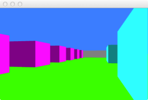
The idea is we are drawing a very simple 3D world by casting viewportWidth number of rays into a scene. These rays are based on the players position, direction, and field of view. Our scene is primitive, constructed by a 2D array populated with integers which will represent different colored cells/blocks while 0 will represent empty space.

We iterate from the left side of the viewport to the right, creating a ray for every column of pixels. Once a ray hits the edge of a cell, we calculate its length. Based on how far away the edge is, we draw a shorter or longer single pixel vertical line centered in the viewport. This is how we will achieve foreshortening.

Since our implementation does not involve any 3D geometry, this technique can be implemented on anything that supports a 2D context. This includes HTML5 canvas and even TI-83 devices.

What really excites me about this method is that the complexity is not dependent on the number of objects in the level, but instead on the number of horizontal pixels in the viewport! Very cool!!

Initial Setup

Inside an empty OpenFrameworks template, you will have a ofApp.h header file. In this file we declare a few variables: pos, right, dir, FOV, and rot all define properties of our player. The width and height variables are aliases and worldMap defines our world.

#pragma once

#include "ofMain.h"

class ofApp : public ofBaseApp{
  private:
  ofVec2f pos;
  ofVec2f right;
  ofVec2f dir;
  float FOV;
  float rot;

  int width;
  int height;
    
  int worldMap[15][24] = {
    {1,1,1,1,1,1,1,1,1,1,1,1,1,1,1,1,1,1,1,1,1,1,1,1},
    {1,0,0,0,0,0,3,3,3,0,0,0,0,0,3,0,0,0,0,0,0,0,0,1},
    {1,0,0,0,0,0,0,0,0,0,0,0,0,0,3,0,0,0,0,0,0,0,0,1},
    {1,0,0,0,3,0,0,3,0,0,0,0,0,0,3,0,0,0,0,0,2,0,0,1},
    {1,0,0,0,3,0,0,0,0,0,0,0,0,0,0,0,0,0,0,0,2,0,0,1},
    {1,0,0,0,3,0,0,0,0,0,0,0,0,0,0,0,0,0,0,0,2,0,0,1},
    {1,0,0,0,3,0,0,0,0,0,0,0,0,0,0,0,0,0,0,0,2,0,0,1},
    {1,0,0,0,3,0,0,0,0,0,2,2,0,0,0,2,2,0,0,0,0,0,0,1},
    {1,0,0,0,3,0,3,0,0,0,2,2,0,0,0,2,2,0,0,0,0,0,0,1},
    {1,0,0,0,3,3,3,0,0,0,2,2,0,0,0,2,2,0,0,0,0,0,0,1},
    {1,0,0,0,0,0,0,0,0,0,0,0,0,0,0,0,0,0,0,0,0,0,0,1},
    {1,0,0,0,0,0,0,0,0,0,0,0,0,0,0,0,0,0,0,0,0,0,0,1},
    {1,0,0,0,0,0,0,3,0,3,0,3,0,3,0,3,0,3,0,3,0,3,0,1},
    {1,0,0,0,0,0,0,0,0,0,0,0,0,0,0,0,0,0,0,0,0,0,0,1},
    {1,1,1,1,1,1,1,1,1,1,1,1,1,1,1,1,1,1,1,1,1,1,1,1}
  };
    
  public:
  void setup();
  void update();
  void draw();
		
  void keyPressed(int key);
  void keyReleased(int key);
  
  ~ofApp();
};

In the setup method of our ofApp.cpp implementation file we assign initial starting values to our player. The position is where the player will be relative to the top left of the array/world. We don’t assign the up and right vectors here since those are set in update() every frame.

void ofApp::setup(){
  pos.set(5, 5);
  FOV = 45;
  rot = PI;
  
  width = ofGetWidth();
  height = ofGetHeight();
}

Setting the Direction and Right Vectors

We need two crucial vectors, the player’s direction and right vector.

In update(), we calculate these vectors based on the scalar rot value. (The keyboard will later drive the rot value, thus rotating the view).

Once we have the direction, we can calculate the perpendicular vector using a perp operation. There is a method which performs this task for you, but I wanted to demonstrate how easy it is here. It just involves swapping the components and negating one.

If our rot value is initially PI, it means we end up looking towards the left inside the world. Since our world is defined by an array it means our y goes positively downward in our world coordinate system.

void ofApp::update(){
  dir.x = cos(rot);
  dir.y = sin(rot);
  
  right.x = -dir.y;
  right.y = dir.x;
}

Drawing a Background

We can now start getting into our render method.

To clear each frame we are going to draw 2 rectangles directly on top of the viewport. The top half of the viewport will be the sky and the bottom will be grass.

void ofApp::draw(){
  // Blue rectangle for the sky
  ofSetColor(64, 128, 255);
  ofRect(0, 0, width, height/2);
  
  // Green rectangle for the ground
  ofSetColor(0, 255, 0);
  ofRect(0, height/2, width, height);

Calculating the Base Length of the Viewing Triangle

The FOV determines the angle from which the rays shoot from the player’s position. The exact center ray will be our player’s direction. Perpendicular to this ray is a line which connects to the far left and far right rays. This all forms a little isosceles triangle. The apex being the player’s position. The base of the triangle is the camera line magnitude which we are trying to calculate. The purpose of getting this is that we need to know how far left and right the rays need to span. The greater the FOV, the wider the rays will span.

Using some simple trigonometry, we can get this length. Note that we divide by two since we’ll be generating the rays in two parts, left side of the direction vector and the right side.

  float camPlaneMag = tan( FOV / 2.0f * (PI / 180.0) );

Generating the Rays

Before we start the main render loop, we declare rayDir which will be re-used for each loop iteration.

  ofVec2f rayDir;

Each iteration of this loop will be responsible for rendering a single pixel vertical line in the viewport. From the far left side of the screen to the far right.

  for(int x = 0; x < width; x++){

For each vertical slice, we need to generate a ray casting out into the scene. We do this by mapping the screen coordinates [0 to width-1] to [-1 to 1]. When x is 0, our ray cast for intersection tests will be collinear with our direction vector.

currCamScale will drive the direction of the rays by taking the result of scaling the right vector.

    float currCamScale = (2.0f * x / float(width)) - 1.0f;

Here is where we generate our rays.

Our right vector is scaled depending on the base of our triangle viewing area. Then we scale it again depending on which slice we are currently rendering. If x = 0, currCamScale maps to -1 which means we are generating the farthest left ray.

Add the resultant vector to the direction vector and this will form our current ray shooting into our scene.

    rayDir.set(dir.x + (right.x * camPlaneMag) * currCamScale, 
               dir.y + (right.y * camPlaneMag) * currCamScale);

Calculating the Magnitude Between Edges

Each ray travels inside a 2D world defined by an array populated with integers. Most of the values are 0 representing empty space. Anything else denotes a wall which is 1×1 unit in dimensions. The integers then help define the ‘cell’ edges. These edges will be used to help us perform intersection tests with the rays.

What we are trying figure out is for each ray, when does it hit an edge? To answer that question we’ll need to figure out some things:

1. What is the magnitude from the players position traveling along the current ray to the nearest x edge (and y edge). Note I say magnitude because we will be working with SCALAR values. I got confused here trying to figure this part out because I kept thinking about vectors.

2. What is the magnitude from one x edge to the next x edge? (And y edge to the next y edge.) We aren’t trying to figure out the vertical/horizontal distance, that’s just a unit of 1. Instead, we need to calculate the hypotenuse of the triangle formed from the ray going from one edge to the other. Again, when calculating the magnitude for x, the horizontal base leg length of the triangle formed will be 1. And when calculating the magnitude for y, the vertical height of the triangle will be 1. Drawing this on paper helps.

Once we have these values we can start running the DDA algorithm. Selecting the nearest x or y edge, testing if that edge has a filled block associated with it, and if not, incrementing some values. We’ll have two scalar values ‘racing’ one another.

Okay, let’s answer the second question first. Based on the direction, what is the magnitude/hypotenuse length from one x edge to another? We know horizontally, the length is 1 unit. That means we need to scale our ray such that the x component will be 1.

What value multiplied by x will result in 1? The answer is the inverse of x! So if we multiply the x component of the ray by 1/x, we’ll need to do the same for y to maintain the ray direction. This gives us a new vector:

v = [ rayDir.x * 1 / rayDir.x , rayDir.y * 1 / rayDir.x]

We already know the result of the calculation for the first component, so we can simplify:

v = [ 1, rayDir.y / rayDir.x ]

Then get the magnitude using the Pythagorean theorem.

    float magBetweenXEdges = ofVec2f(1, rayDir.y * (1.0 / rayDir.x) ).length();
    float magBetweenYEdges = ofVec2f(rayDir.x * (1.0 / rayDir.y), 1).length();

Calculating the Starting Magnitude

For this we have to calculate the length from the player’s position to the nearest x and y edges. To do this, we get the relative position from within the cell then use that as a scale for the magnitude between the edges.

Here we keep track of which direction the ray is going by setting dirStepX which will be used to jump from cell to cell in the correct direction.

For x, we have a triangle with a base horizontal length of 1 and some magnitude for its hypotenuse which we recently figured out. Now, based on the relative position of the user within a cell, how long is the hypotenuse of this triangle?

If the x position of the player was 0.2:

magToXedge = (0 + 1 - 0.2) * magBetweenXedges
           = 0.8 * magBetweenXedges

This means we are 80% away from the closest x edge, thus we need 80% of the hypotenuse. The same method is used to calculate the starting position of the y edge.

    if(rayDir.x > 0){
      magToXedge = (worldIndexX + 1.0 - pos.x) * magBetweenXEdges;
      dirStepX = 1;
    }
    else{
      magToXedge = (pos.x - worldIndexX) * magBetweenXEdges;
      dirStepX = -1;
    }

    if(rayDir.y > 0){
      magToYedge = (worldIndexY + 1.0 - pos.y) * magBetweenYEdges;
      dirStepY = 1;
    }
    else{
      magToYedge = (pos.y - worldIndexY) * magBetweenYEdges;
      dirStepY = -1;
    }

Running the Search

Here x and y values ‘race’. If one length is less than the other, we increase the shortest, increment 1 unit in that direction and check again. We end the loop as soon as we find a non-empty cell edge.

Note, we keep track of not only the last cell we were working with, but also which edge (x or y) that we hit with sideHit.

    int sideHit;

    do{
      if(magToXedge < magToYedge){
        magToXedge += magBetweenXEdges;
        worldIndexX += dirStepX;
        sideHit = 0;
      }
      else{
        magToYedge += magBetweenYEdges;
        worldIndexY += dirStepY;
        sideHit = 1;
      }
    }while(worldMap[worldIndexX][worldIndexY] == 0);

Selecting a Color & Lighting

We kept track of the non-empty index we hit, so we can use this to index into the map and get the associated color for the cell.

    ofColor wallColor;
    switch(worldMap[worldIndexX][worldIndexY]){
      case 1:wallColor = ofColor(255,255,255);break;
      case 2:wallColor = ofColor(0,255,255);break;
      case 3:wallColor = ofColor(255,0,255);break;
    }

If all faces of the walls were a solid color, it would be difficult to determine edges and where the walls were in relation to each other. So to provide a very rudimentary form of lighting, any time the rays hit an x edge, we darken the current color.

    wallColor = sideHit == 0 ? wallColor : wallColor/2.0f;
    ofSetColor(wallColor);

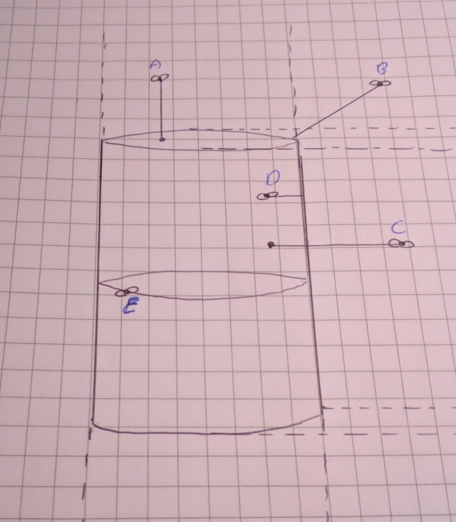
Preventing Distortion

The farther the wall is from the player, the smaller the vertical slice needs to be on the screen. Keep in mind when viewing a wall/plane dead on, the length of the rays further out will be longer resulting in shorter ‘scanlines’. This isn’t desired since it will warp our representation of the world.

***Update***
After I posted this I was e-mailed how this part works, here’s an image to help clarify things:

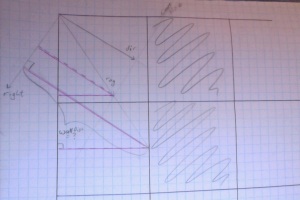
Essentially, we take the base of the ‘lower’ triangle and divide it by the base of the ‘upper’ triangle. This value is actually the same proportionally as the perpendicular to camera line to the direction vector.

    float wallDist;

    if(sideHit == 0){
      wallDist = fabs((worldIndexX - pos.x + (1.0 - dirStepX) / 2.0) / rayDir.x);
    }
    else{
      wallDist = fabs((worldIndexY - pos.y + (1.0 - dirStepY) / 2.0) / rayDir.y);
    }

Calculating Line Height

If a ray was 1 unit from the wall, we draw a line that fills the entire length of the screen.

To provide a proper FPS feel, we center the vertical lines in screen space along Y. The middle of the cells will be at eye height.

To calculate how long the vertical line needs to be on the screen, we divide the viewport height by the distance from the wall. So if the wall was 1 unit from the player, it will fill up the entire vertical slide.

At this point we need to center our line height in our viewport line. Draw two vertical lines down, the smaller one centered next to the larger one. To get the position of top of the smaller one relative to the larger one, you just have to divide both lines halfway horizontally then subtract from that the half that remained from the smaller line. This gives us the starting point for the line we have to draw.

    float lineHeight = height/wallDist;
    float startY = height/2.0 - lineHeight/2.0;

Rendering a Slice

We finish our render loop by drawing a single pixel width vertical line for this x scanline iteration and we center it in the viewport. You can always clamp the lines to the bottom of the screen and make the player feel like they are mouse in a maze (:

    ofLine(x, startY, x, startY + lineHeight);
  }// finish loop
}// finish draw()

Keyboard Control

I’m still learning OpenFrameworks, so my implementation for keyboard control works, but it’s a hack. I’m too embarrassed to post the code until I resolve the issue I’m dealing with. In the mean time, I leave the task of updating position and rotation of the player up to the reader.

References

[1] http://www.permadi.com/tutorial/raycast/index.html
[2] http://lodev.org/cgtutor/raycasting.html
[3] http://en.wikipedia.org/wiki/Ray_casting